pacman::p_load(tmap, sf, tidyverse, knitr)In-class Exercise 1: My First Date with Geospatial Data Science
The Task
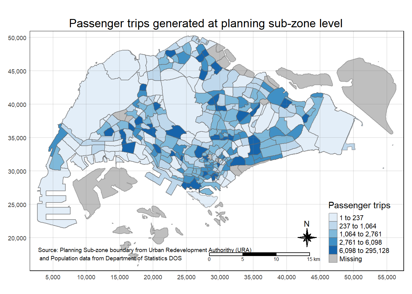
In this in-class exercise, you are required to prepare a choropleth map showing the distribution of passenger trips at planning sub-zone by integrating Passenger Volume by Origin Destination Bus Stops and bus stop data sets downloaded from LTA DataMall and Planning Sub-zone boundary of URA Master Plan 2019 downloaded from data.gov.sg.
The specific task of this in-class exercise are as follows:
to import Passenger Volume by Origin Destination Bus Stops data set downloaded from LTA DataMall in to RStudio environment,
to import geospatial data in ESRI shapefile format into sf data frame format,
to perform data wrangling by using appropriate functions from tidyverse and sf pakcges, and
to visualise the distribution of passenger trip by using tmap methods and functions.
Getting Started
Three R packages will be used in this in-class exercise, they are:
tidyverse for non-spatial data handling,
sf for geospatial data handling,
tmap for thematic mapping, and
knitr for creating html table.
Importing the OD data
Firstly, we will import the Passenger Volume by Origin Destination Bus Stops data set downloaded from LTA DataMall by using read_csv() of readr package.
odbus <- read_csv("data/aspatial/origin_destination_bus_202308.csv")Rows: 5709512 Columns: 7
── Column specification ────────────────────────────────────────────────────────
Delimiter: ","
chr (5): YEAR_MONTH, DAY_TYPE, PT_TYPE, ORIGIN_PT_CODE, DESTINATION_PT_CODE
dbl (2): TIME_PER_HOUR, TOTAL_TRIPS
ℹ Use `spec()` to retrieve the full column specification for this data.
ℹ Specify the column types or set `show_col_types = FALSE` to quiet this message.A quick check of odbus tibble data frame shows that the values in OROGIN_PT_CODE and DESTINATON_PT_CODE are in numeric data type.
glimpse(odbus)Rows: 5,709,512
Columns: 7
$ YEAR_MONTH <chr> "2023-08", "2023-08", "2023-08", "2023-08", "2023-…
$ DAY_TYPE <chr> "WEEKDAY", "WEEKENDS/HOLIDAY", "WEEKENDS/HOLIDAY",…
$ TIME_PER_HOUR <dbl> 16, 16, 14, 14, 17, 17, 17, 17, 7, 17, 14, 10, 10,…
$ PT_TYPE <chr> "BUS", "BUS", "BUS", "BUS", "BUS", "BUS", "BUS", "…
$ ORIGIN_PT_CODE <chr> "04168", "04168", "80119", "80119", "44069", "4406…
$ DESTINATION_PT_CODE <chr> "10051", "10051", "90079", "90079", "17229", "1722…
$ TOTAL_TRIPS <dbl> 7, 2, 3, 10, 5, 4, 3, 22, 3, 3, 7, 1, 3, 1, 3, 1, …odbus$ORIGIN_PT_CODE <- as.factor(odbus$ORIGIN_PT_CODE)
odbus$DESTINATION_PT_CODE <- as.factor(odbus$DESTINATION_PT_CODE) Notice that both of them are in factor data type now.
glimpse(odbus)Rows: 5,709,512
Columns: 7
$ YEAR_MONTH <chr> "2023-08", "2023-08", "2023-08", "2023-08", "2023-…
$ DAY_TYPE <chr> "WEEKDAY", "WEEKENDS/HOLIDAY", "WEEKENDS/HOLIDAY",…
$ TIME_PER_HOUR <dbl> 16, 16, 14, 14, 17, 17, 17, 17, 7, 17, 14, 10, 10,…
$ PT_TYPE <chr> "BUS", "BUS", "BUS", "BUS", "BUS", "BUS", "BUS", "…
$ ORIGIN_PT_CODE <fct> 04168, 04168, 80119, 80119, 44069, 44069, 20281, 2…
$ DESTINATION_PT_CODE <fct> 10051, 10051, 90079, 90079, 17229, 17229, 20141, 2…
$ TOTAL_TRIPS <dbl> 7, 2, 3, 10, 5, 4, 3, 22, 3, 3, 7, 1, 3, 1, 3, 1, …Extracting the study data
origin7_9 <- odbus %>%
  filter(DAY_TYPE == "WEEKDAY") %>%
  filter(TIME_PER_HOUR >= 7 &
           TIME_PER_HOUR <= 9) %>%
  group_by(ORIGIN_PT_CODE) %>%
  summarise(TRIPS = sum(TOTAL_TRIPS))
It should look similar to the data table below.
kable(head(origin7_9))| ORIGIN_PT_CODE | TRIPS |
|---|---|
| 01012 | 1617 |
| 01013 | 813 |
| 01019 | 1620 |
| 01029 | 2383 |
| 01039 | 2727 |
| 01059 | 1415 |
We will save the output in rds format for future used.
write_rds(origin7_9, "data/origin7_9.rds")The code chunk below will be used to import the save origin7_9.rds into R environment.
origin7_9 <- read_rds("data/origin7_9.rds")Working with Geospatial Data
In this section, you are required to import two shapefile into RStudio, they are:
BusStop: This data provides the location of bus stop as at last quarter of 2022.
MPSZ-2019: This data provides the sub-zone boundary of URA Master Plan 2019.
Importing geospatial data
busstop <- st_read(dsn = "data/geospatial",
                   layer = "BusStop") %>%
  st_transform(crs = 3414)
Reading layer `BusStop' from data source
`C:\czx0727\ISSS624_\in_class_ex1\data\geospatial' using driver `ESRI Shapefile'
Simple feature collection with 5161 features and 3 fields
Geometry type: POINT
Dimension: XY
Bounding box: xmin: 3970.122 ymin: 26482.1 xmax: 48284.56 ymax: 52983.82
Projected CRS: SVY21glimpse(busstop)Rows: 5,161
Columns: 4
$ BUS_STOP_N <chr> "22069", "32071", "44331", "96081", "11561", "66191", "2338…
$ BUS_ROOF_N <chr> "B06", "B23", "B01", "B05", "B05", "B03", "B02A", "B02", "B…
$ LOC_DESC <chr> "OPP CEVA LOGISTICS", "AFT TRACK 13", "BLK 239", "GRACE IND…
$ geometry <POINT [m]> POINT (13576.31 32883.65), POINT (13228.59 44206.38),…mpsz <- st_read(dsn = "data/geospatial",
layer = "MPSZ-2019") %>%
st_transform(crs = 3414)Reading layer `MPSZ-2019' from data source
`C:\czx0727\ISSS624_\in_class_ex1\data\geospatial' using driver `ESRI Shapefile'
Simple feature collection with 332 features and 6 fields
Geometry type: MULTIPOLYGON
Dimension: XY
Bounding box: xmin: 103.6057 ymin: 1.158699 xmax: 104.0885 ymax: 1.470775
Geodetic CRS: WGS 84The structure of mpsz sf tibble data frame should look as below.
glimpse(mpsz)Rows: 332
Columns: 7
$ SUBZONE_N <chr> "MARINA EAST", "INSTITUTION HILL", "ROBERTSON QUAY", "JURON…
$ SUBZONE_C <chr> "MESZ01", "RVSZ05", "SRSZ01", "WISZ01", "MUSZ02", "MPSZ05",…
$ PLN_AREA_N <chr> "MARINA EAST", "RIVER VALLEY", "SINGAPORE RIVER", "WESTERN …
$ PLN_AREA_C <chr> "ME", "RV", "SR", "WI", "MU", "MP", "WI", "WI", "SI", "SI",…
$ REGION_N <chr> "CENTRAL REGION", "CENTRAL REGION", "CENTRAL REGION", "WEST…
$ REGION_C <chr> "CR", "CR", "CR", "WR", "CR", "CR", "WR", "WR", "CR", "CR",…
$ geometry <MULTIPOLYGON [m]> MULTIPOLYGON (((33222.98 29..., MULTIPOLYGON (…Geospatial data wrangling
Combining Busstop and mpsz
busstop_mpsz <- st_intersection(busstop, mpsz) %>%
  select(BUS_STOP_N, SUBZONE_C) %>%
  st_drop_geometry()
Warning: attribute variables are assumed to be spatially constant throughout
all geometriesBefore moving to the next step, it is wise to save the output into rds format.
write_rds(busstop_mpsz, "data/busstop_mpsz.csv") origin_data <- left_join(origin7_9 , busstop_mpsz,
by = c("ORIGIN_PT_CODE" = "BUS_STOP_N")) %>%
rename(ORIGIN_BS = ORIGIN_PT_CODE,
ORIGIN_SZ = SUBZONE_C)Before continue, it is a good practice for us to check for duplicating records.
duplicate <- origin_data %>%
  group_by_all() %>%
  filter(n()>1) %>%
  ungroup()
If duplicated records are found, the code chunk below will be used to retain the unique records.
origin_data <- unique(origin_data)mpsz_origtrip <- left_join(mpsz,
origin_data,
by = c("SUBZONE_C" = "ORIGIN_SZ"))Choropleth Visualisation
tm_shape(mpsz_origtrip)+
  tm_fill("TRIPS",
          style = "quantile",
          palette = "Blues",
          title = "Passenger trips") +
  tm_layout(main.title = "Passenger trips generated at planning sub-zone level",
            main.title.position = "center",
            main.title.size = 1.2,
            legend.height = 0.45,
            legend.width = 0.35,
            frame = TRUE) +
  tm_borders(alpha = 0.5) +
  tm_compass(type="8star", size = 2) +
  tm_scale_bar() +
  tm_grid(alpha =0.2) +
  tm_credits("Source: Planning Sub-zone boundary from Urban Redevelopment Authorithy (URA)\n and Population data from Department of Statistics DOS",
             position = c("left", "bottom"))