pacman::p_load(sf, spdep, tmap, tidyverse)Hands-on Exercise 2.2 Global Measures of Spatial Autocorrelation
Overview
I will learn how to compute Global and Local Measure of Spatial Autocorrelation (GLSA) by using spdep package.
Getting Started
Setting the Analytical Tools
Two data sets will be used in this hands-on exercise, they are:
Hunan province administrative boundary layer at county level. This is a geospatial data set in ESRI shapefile format.
Hunan_2012.csv: This csv file contains selected Hunan's local development indicators in 2012.
Getting the Data Into R Environment
The code chunk below uses st_read() of sf package to import Hunan shapefile into R. The imported shapefile will be simple features Object of sf.
Import shapefile into r environment
hunan <- st_read(dsn = "data/geospatial",
                 layer = "Hunan")
Reading layer `Hunan' from data source
`C:\czx0727\ISSS624_\hands_on_ex2\data\geospatial' using driver `ESRI Shapefile'
Simple feature collection with 88 features and 7 fields
Geometry type: POLYGON
Dimension: XY
Bounding box: xmin: 108.7831 ymin: 24.6342 xmax: 114.2544 ymax: 30.12812
Geodetic CRS: WGS 84Import csv file into r environment
hunan2012 <- read_csv("data/aspatial/Hunan_2012.csv")Rows: 88 Columns: 29
── Column specification ────────────────────────────────────────────────────────
Delimiter: ","
chr (2): County, City
dbl (27): avg_wage, deposite, FAI, Gov_Rev, Gov_Exp, GDP, GDPPC, GIO, Loan, ...
ℹ Use `spec()` to retrieve the full column specification for this data.
ℹ Specify the column types or set `show_col_types = FALSE` to quiet this message.Performing relational join
hunan <- left_join(hunan,hunan2012) %>%
  select(1:4, 7, 15)
Joining with `by = join_by(County)`Visualising Regional Development Indicator
I prepare a basemap and a choropleth map showing the distribution of GDPPC 2012 by using qtm() of tmap package.
equal <- tm_shape(hunan) +
  tm_fill("GDPPC",
          n = 5,
          style = "equal") +
  tm_borders(alpha = 0.5) +
  tm_layout(main.title = "Equal interval classification")

quantile <- tm_shape(hunan) +
  tm_fill("GDPPC",
          n = 5,
          style = "quantile") +
  tm_borders(alpha = 0.5) +
  tm_layout(main.title = "Equal quantile classification")

tmap_arrange(equal,
             quantile,
             asp=1,
             ncol=2)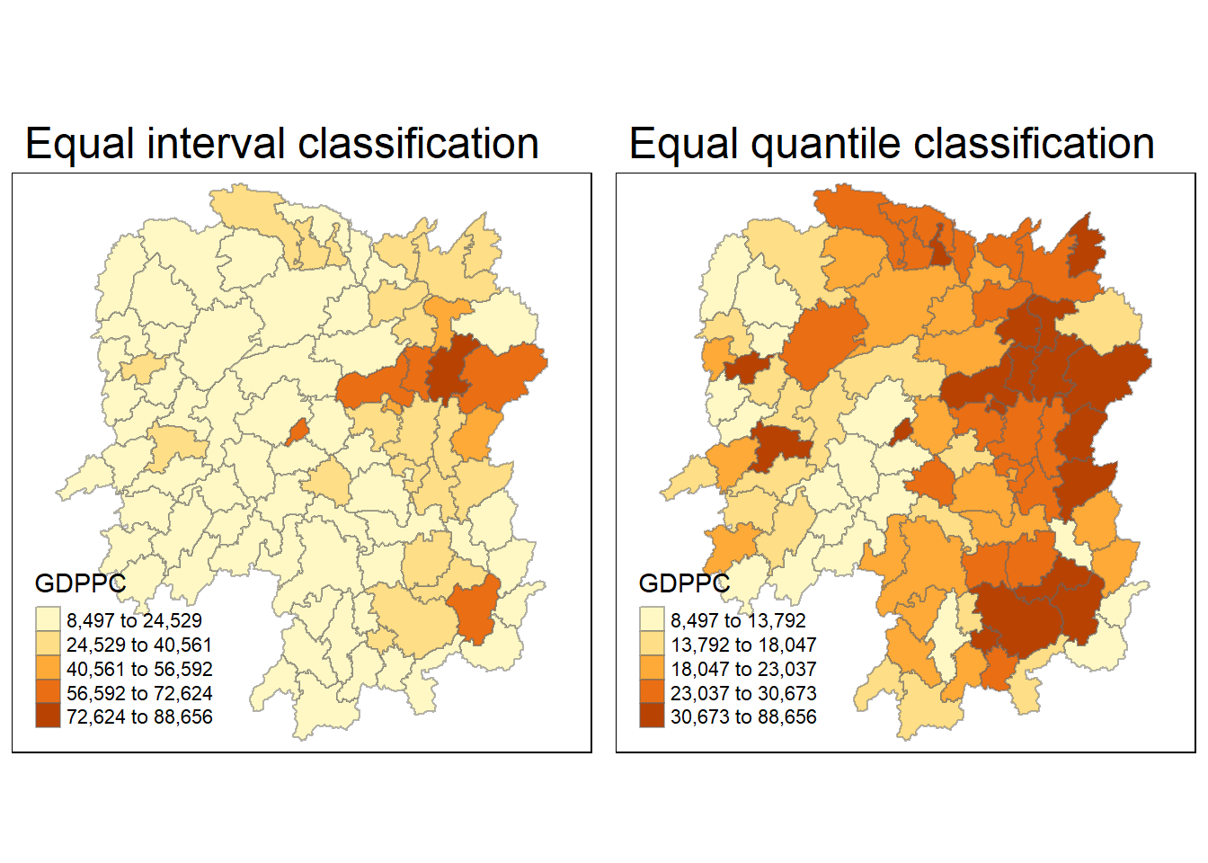
Global Spatial Autocorrelation
Computing Contiguity Spatial Weights
In the code chunk below, poly2nb() of spdep package is used to compute contiguity weight matrices for the study area. This function builds a neighbours list based on regions with contiguous boundaries.
wm_q <- poly2nb(hunan,
                queen=TRUE)
summary(wm_q)
Neighbour list object:
Number of regions: 88
Number of nonzero links: 448
Percentage nonzero weights: 5.785124
Average number of links: 5.090909
Link number distribution:
1 2 3 4 5 6 7 8 9 11
2 2 12 16 24 14 11 4 2 1
2 least connected regions:
30 65 with 1 link
1 most connected region:
85 with 11 linksRow-standardised weights matrix
rswm_q <- nb2listw(wm_q,
                   style="W",
                   zero.policy = TRUE)
rswm_q
Characteristics of weights list object:
Neighbour list object:
Number of regions: 88
Number of nonzero links: 448
Percentage nonzero weights: 5.785124
Average number of links: 5.090909
Weights style: W
Weights constants summary:
n nn S0 S1 S2
W 88 7744 88 37.86334 365.9147Global Spatial Autocorrelation: Moran's I
In this section, I will learn how to perform Moran's I statistics testing by using moran.test() of spdep.
Maron's I test
moran.test(hunan$GDPPC,
           listw=rswm_q,
           zero.policy = TRUE,
           na.action=na.omit)
    Moran I test under randomisation

data:  hunan$GDPPC
weights: rswm_q

Moran I statistic standard deviate = 4.7351, p-value = 1.095e-06
alternative hypothesis: greater
sample estimates:
Moran I statistic       Expectation          Variance
      0.300749970      -0.011494253       0.004348351
** Conclusion
The Moran’s I test suggests strong evidence against the null hypothesis of spatial randomness (p-value = 1.095e-06). The Moran’s I statistic of 0.3007 indicates a significant positive spatial autocorrelation in the variable ‘GDPPC’ within the study area. Areas in this region with similar GDPPC values tend to be spatially clustered or adjacent to each other more often than expected by random chance.
Computing Monte Carlo Moran's I
The code chunk below performs permutation test for Moran's I statistic by using moran.mc() of spdep. A total of 1000 simulation will be performed.
set.seed(1234)
bperm= moran.mc(hunan$GDPPC,
                listw=rswm_q,
                nsim=999,
                zero.policy = TRUE,
                na.action=na.omit)
bperm
    Monte-Carlo simulation of Moran I

data:  hunan$GDPPC
weights: rswm_q
number of simulations + 1: 1000

statistic = 0.30075, observed rank = 1000, p-value = 0.001
alternative hypothesis: greater
** Conclusion
The permutation test for Moran’s I statistic indicates strong evidence against the null hypothesis of spatial randomness. The observed Moran’s I value (0.30075) falls within the highest ranks of the simulated values, and the small p-value (0.001) suggests that this value is significantly greater than what would be expected by chance alone. Therefore, it supports the conclusion that there is a significant positive spatial autocorrelation in the ‘GDPPC’ variable within the study area. Areas with similar GDPPC values tend to be spatially clustered or adjacent to each other more often than expected by random chance.
Visualising Monte Carlo Moran's I
In the code chunk below hist() and abline() of R Graphics are used.
mean(bperm$res[1:999])[1] -0.01504572var(bperm$res[1:999])[1] 0.004371574summary(bperm$res[1:999]) Min. 1st Qu. Median Mean 3rd Qu. Max.
-0.18339 -0.06168 -0.02125 -0.01505 0.02611 0.27593 hist(bperm$res,
freq=TRUE,
breaks=20,
xlab="Simulated Moran's I")
abline(v=0,
col="red") 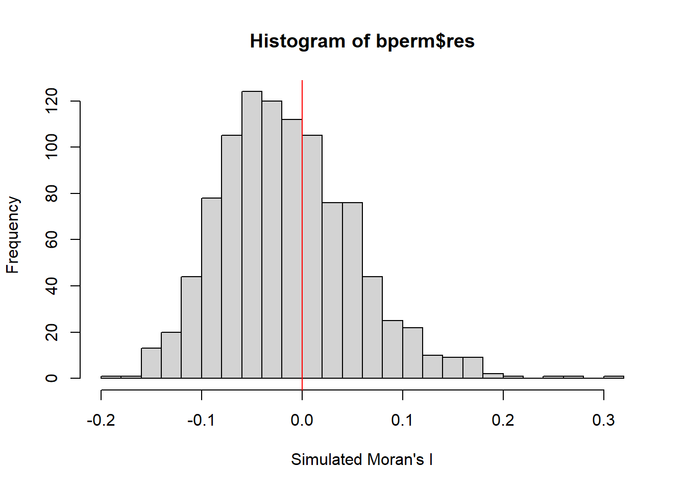
** Observation
Skewed distribution that is of right skewed. It peaks at -0.05
Plot values using ggplot:
bperm <- list(
  res = rnorm(1000),
  statistic = 0.30075
)


plot_data <- data.frame(
  Simulation = 1:length(bperm$res),
  Moran_I = bperm$res
)


plot <- ggplot(plot_data, aes(x = Simulation, y = Moran_I)) +
  geom_point(color = "blue", alpha = 0.6) +
  geom_hline(yintercept = bperm$statistic, linetype = "dashed", color = "red") +
  labs(
    title = "Permutation Test for Moran's I",
    x = "Simulation",
    y = "Moran's I Value"
  ) +
  theme_minimal()

plot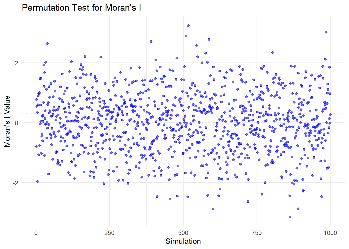
Global Spatial Autocorrelation: Geary's
I will learn how to perform Geary's c statistics testing by using appropriate functions of spdep package.
Geary's C test
The code chunk below performs Geary's C test for spatial autocorrelation by using geary.test() of spdep.
geary.test(hunan$GDPPC, listw=rswm_q)
    Geary C test under randomisation

data:  hunan$GDPPC
weights: rswm_q

Geary C statistic standard deviate = 3.6108, p-value = 0.0001526
alternative hypothesis: Expectation greater than statistic
sample estimates:
Geary C statistic       Expectation          Variance
        0.6907223         1.0000000         0.0073364
** Conclusion
Given the low p-value, we can conclude that there is significant evidence to reject the null hypothesis of spatial randomness. We have sufficient evidence to conclude that the alternative hypothesis that there is spatial autocorrelation present in the variable “hunan$GDPPC.” Moreover, the Geary C statistic being substantially lower than the expected value under the null hypothesis further supports this conclusion.
Computing Monte Carlo Geary's C
The code chunk below performs permutation test for Geary's C statistic by using geary.mc() of spdep.
set.seed(1234)
bperm=geary.mc(hunan$GDPPC,
               listw=rswm_q,
               nsim=999)
bperm
    Monte-Carlo simulation of Geary C

data:  hunan$GDPPC
weights: rswm_q
number of simulations + 1: 1000

statistic = 0.69072, observed rank = 1, p-value = 0.001
alternative hypothesis: greater
**Conclusion
The very low p-value (0.001) suggests strong evidence against the null hypothesis of spatial randomness. Instead, it supports the alternative hypothesis that there is significant spatial autocorrelation present in the variable “hunan$GDPPC.”
Furthermore, the observed rank of 1 among the 1000 simulations indicates that your observed statistic is at the extreme end of the simulated distribution. This strengthens the evidence that the observed spatial autocorrelation is significantly higher than what would be expected by chance.
Visualising the Monte Carlo Geary's C
We plot a histogram to reveal the distribution of the simulated values by using the code chunk below.
mean(bperm$res[1:999])[1] 1.004402var(bperm$res[1:999])[1] 0.007436493summary(bperm$res[1:999]) Min. 1st Qu. Median Mean 3rd Qu. Max.
0.7142 0.9502 1.0052 1.0044 1.0595 1.2722 hist(bperm$res, freq=TRUE, breaks=20, xlab="Simulated Geary c")
abline(v=1, col="red") 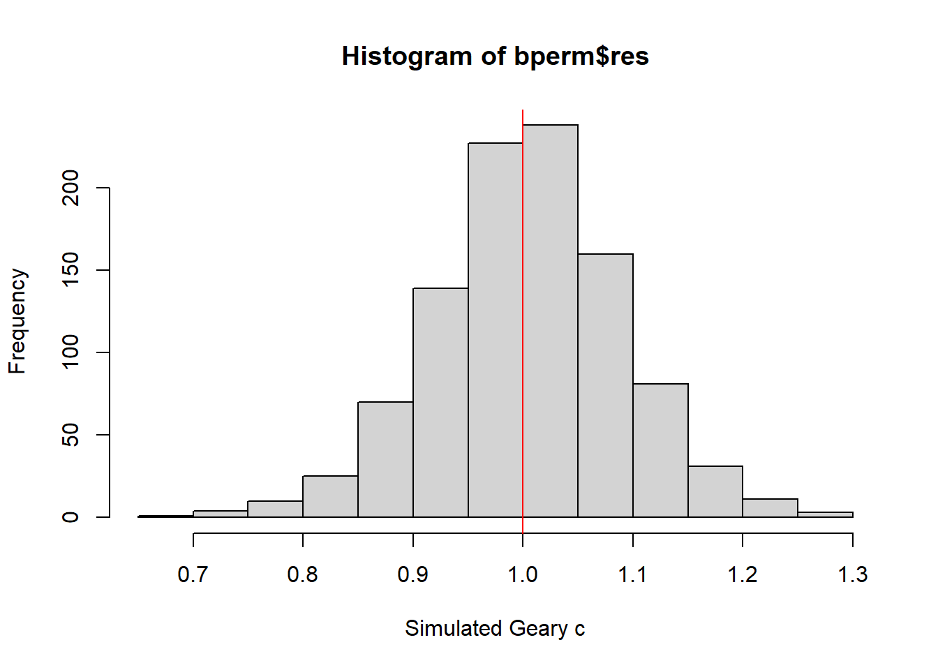
** Observation
Skewed distribution that is of left skewed. It peaks at 1.05
Spatial Correlogram
Compute Moran's I correlogram
In the code chunk below, sp.correlogram() of spdep package is used to compute a 6-lag spatial correlogram of GDPPC. The global spatial autocorrelation used in Moran's I. The plot() of base Graph is then used to plot the output.
MI_corr <- sp.correlogram(wm_q,
                          hunan$GDPPC,
                          order=6,
                          method="I",
                          style="W")
plot(MI_corr)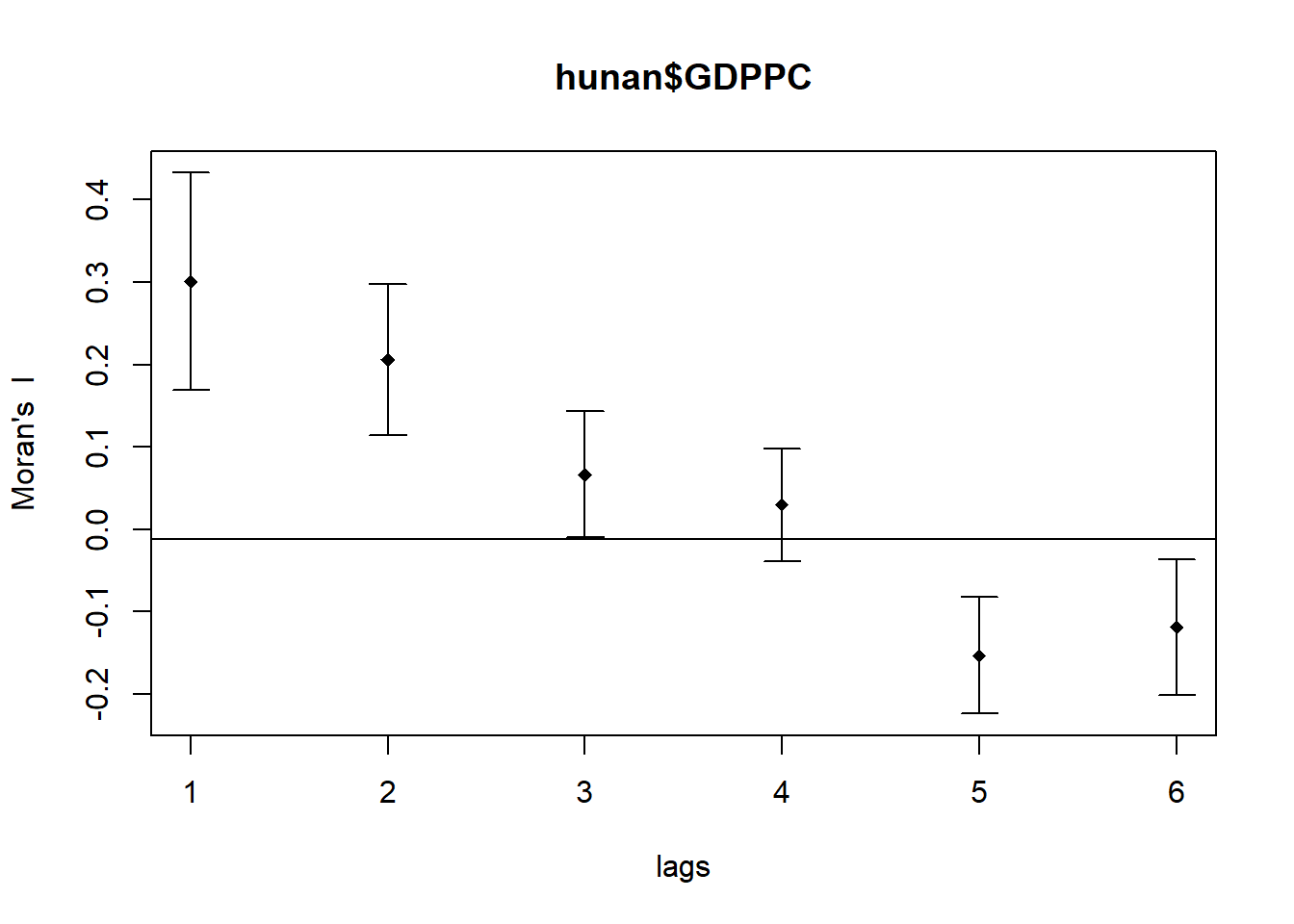
Full analysis report
print(MI_corr)Spatial correlogram for hunan$GDPPC
method: Moran's I
estimate expectation variance standard deviate Pr(I) two sided
1 (88) 0.3007500 -0.0114943 0.0043484 4.7351 2.189e-06 ***
2 (88) 0.2060084 -0.0114943 0.0020962 4.7505 2.029e-06 ***
3 (88) 0.0668273 -0.0114943 0.0014602 2.0496 0.040400 *
4 (88) 0.0299470 -0.0114943 0.0011717 1.2107 0.226015
5 (88) -0.1530471 -0.0114943 0.0012440 -4.0134 5.984e-05 ***
6 (88) -0.1187070 -0.0114943 0.0016791 -2.6164 0.008886 **
---
Signif. codes: 0 '***' 0.001 '**' 0.01 '*' 0.05 '.' 0.1 ' ' 1**Conclusion
In this output, the Moran’s I statistics at various distance bands are presented.
The Moran’s I values at different distance classes vary and show varying levels of significance.
For instance, at the 1st and 2nd distance bands, the Moran’s I values are significantly positive with very low p-values (***), indicating strong positive spatial autocorrelation.
At farther distance bands (e.g., 5th and 6th), the Moran’s I values become negative and remain significant (**, *), suggesting negative spatial autocorrelation or dissimilarity among more distant areas.
Compute Geary's C correlogram and plot
In the code chunk below, sp.correlogram() of spdep package is used to compute a 6-lag spatial correlogram of GDPPC. The global spatial autocorrelation used in Geary's C. The plot() of base Graph is then used to plot the output.
GC_corr <- sp.correlogram(wm_q,
                          hunan$GDPPC,
                          order=6,
                          method="C",
                          style="W")
plot(GC_corr)
print(GC_corr)Spatial correlogram for hunan$GDPPC
method: Geary's C
estimate expectation variance standard deviate Pr(I) two sided
1 (88) 0.6907223 1.0000000 0.0073364 -3.6108 0.0003052 ***
2 (88) 0.7630197 1.0000000 0.0049126 -3.3811 0.0007220 ***
3 (88) 0.9397299 1.0000000 0.0049005 -0.8610 0.3892612
4 (88) 1.0098462 1.0000000 0.0039631 0.1564 0.8757128
5 (88) 1.2008204 1.0000000 0.0035568 3.3673 0.0007592 ***
6 (88) 1.0773386 1.0000000 0.0058042 1.0151 0.3100407
---
Signif. codes: 0 '***' 0.001 '**' 0.01 '*' 0.05 '.' 0.1 ' ' 1**Conclusion
n this output, the Geary’s C statistics at various distance bands are presented.
The values in the “estimate” column fluctuate across distance classes, indicating variations in the degree of spatial autocorrelation at different distances.
At the 1st and 2nd distance bands, the Geary’s C values are significantly lower than 1 (***), indicating significant spatial autocorrelation.
As the distance bands increase (e.g., 5th and 6th), Geary’s C values move closer to or above 1, suggesting weaker evidence of spatial autocorrelation, although the 5th distance band still shows significant autocorrelation (***).